
Ray is an open-source unified compute framework that simplifies scaling AI and Python workloads in a distributed environment. Since we introduced support for running Ray on Databricks, we’ve witnessed numerous customers successfully deploying their machine learning use cases, which range from forecasting and deep reinforcement learning to fine-tuning LLMs.
With the release of Ray version 2.8.0, we are delighted to announce the addition of autoscaling support for Ray on Databricks. Autoscaling is essential because it allows resources to dynamically adjust to fluctuating demands. This ensures optimal performance and cost-efficiency, as processing needs can vary significantly over time, and it helps maintain a balance between computational power and expenses without requiring manual intervention.
Ray autoscaling on Databricks can add or remove worker nodes as needed, leveraging the Spark framework to enhance scalability, cost-effectiveness, and responsiveness in distributed computing environments. This integrated approach is far simpler than the alternative of implementing OSS autoscaling by eliminating the need for defining complex permissions, cloud initialization scripts, and logging configurations. With a fully-managed, production-capable, and integrated autoscaling solution, you can greatly reduce the complexity and cost of your Ray workloads.
Create Ray cluster on Databricks with autoscaling enabled
To get started, simply install the latest version of Ray
# Install Ray with the 'default','tune' extensions for
# Ray dashboard, and tuning support
%pip install ray[default,tune]>=2.8.0
The next step is to establish the configuration for the Ray cluster that we’re going to be starting by using the `ray.util.spark.setup_ray_cluster() ` function. In order to leverage autoscaling functionality, specify the maximum number of worker nodes that the Ray cluster can use, define the allocated compute resources, and set the Autoscale flag to True. Additionally, it is critical to ensure that the Databricks cluster has been started with autoscaling enabled. For more details, please refer to the documentation.
Once these parameters have been set, when you initialize the Ray cluster, autoscaling will function exactly as Databricks autoscaling does. Below is an example of setting up a Ray cluster with the ability to autoscale.
from ray.util.spark import setup_ray_cluster
setup_ray_cluster(
 num_worker_nodes,#set to max number of nodes to Autoscale
 num_cpus_head_node,# set to the cores used in the driver node
 num_gpus_head_node, # set for GPU enabled cluster
 num_cpus_per_node,# cores added from each worker node
 num_gpus_per_node, #set for GPU enabled cluster
 autoscale = True #set only for clusters with Auto Scaling Enabled
)
This feature is compatible with any Databricks cluster running Databricks Runtime version 14.0 or above.
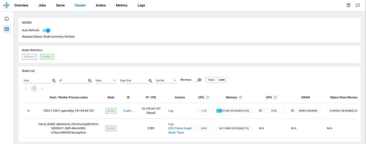
To learn more about the parameters that are available for configuring a Ray cluster on Spark, please refer to the setup_ray_cluster documentation. Once the Ray cluster is initialized, the Ray head node will show up on the Ray Dashboard.
from ray.util.spark import setup_ray_cluster, shutdown_ray_cluster

ray_conf = setup_ray_cluster(
     num_worker_nodes= 4,
     num_cpus_head_node=3,
     num_cpus_per_node=4,
     autoscale = True
)
When a job is submitted to the Ray cluster, the Ray Autoscaler API requests resources from the Spark cluster by submitting tasks with the necessary CPU and GPU compute requirements. The Spark scheduler scales up worker nodes if the current cluster resources cannot meet the task’s compute demands and scales down the cluster when tasks are completed and no additional tasks are pending. You can control the scale-up and scale-down velocity by adjusting the autoscale_upscaling_speed and autoscale_idle_timeout_minutes parameters. For additional details about these control parameters, please refer to the documentation. Once the process is completed, Ray releases all of the allocated resources back to the Spark cluster for other tasks or for downscaling, ensuring efficient utilization of resources.
Let’s walk through a hyperparameter tuning example to demonstrate the autoscaling process. In this example, we’ll train a PyTorch model on the CIFAR10 dataset. We’ve adapted the code from the Ray documentation, which you can find here.
We’ll begin by defining the PyTorch model we want to tune.
import torch.nn as nn
import torch.nn.functional as F


class Net(nn.Module):
 def __init__(self, l1=120, l2=84):
  super(Net, self).__init__()
  self.conv1 = nn.Conv2d(3, 6, 5)
  self.pool = nn.MaxPool2d(2, 2)
  self.conv2 = nn.Conv2d(6, 16, 5)
  self.fc1 = nn.Linear(16 * 5 * 5, l1)
  self.fc2 = nn.Linear(l1, l2)
  self.fc3 = nn.Linear(l2, 10)

 def forward(self, x):
  x = self.pool(F.relu(self.conv1(x)))
  x = self.pool(F.relu(self.conv2(x)))
  x = x.view(-1, 16 * 5 * 5)
  x = F.relu(self.fc1(x))
  x = F.relu(self.fc2(x))
  x = self.fc3(x)
  return x
We wrap the data loaders in their own function and pass a global data directory. This way we can share a data directory between different trials.
import torchvision
import torchvision.transforms as transforms
from filelock import FileLock


def load_data(data_dir="./data"):
    transform = transforms.Compose(
        [transforms.ToTensor(), transforms.Normalize((0.5, 0.5, 0.5), (0.5, 0.5, 0.5))]
    )

    # We add FileLock here because multiple workers will want to
    # download data, and this may cause overwrites since
    # DataLoader is not threadsafe.
    with FileLock(os.path.expanduser("~/.data.lock")):
        trainset = torchvision.datasets.CIFAR10(
            root=data_dir, train=True, download=True, transform=transform
        )

        testset = torchvision.datasets.CIFAR10(
            root=data_dir, train=False, download=True, transform=transform
        )

    return trainset, testset
Next, we can define a function that will ingest a config and run a single training loop for the torch model. At the conclusion of each trial, we checkpoint the weights and report the evaluated loss using the `train, report` API. This is done so that the scheduler can stop ineffectual trials that do not improve the model’s loss characteristics.
import os
import torch
import torch.optim as optim
from torch.utils.data import random_split

import ray
from ray import train, tune
from ray.train import Checkpoint


def train_cifar(config, loc):  # location to store the checkpoints
    net = Net(config["l1"], config["l2"])
    # check whether to load in CPU or GPU
    device = "cpu"
    if torch.cuda.is_available():
        device = "cuda:0"
    net.to(device)

    criterion = nn.CrossEntropyLoss()
    optimizer = optim.SGD(net.parameters(), lr=config["lr"], momentum=0.9)

    # load the Dataset
    data_dir = os.path.abspath("./data")
    trainset, testset = load_data(data_dir)

    test_abs = int(len(trainset) * 0.8)
    train_subset, val_subset = random_split(
        trainset, [test_abs, len(trainset) - test_abs]
    )

    trainloader = torch.utils.data.DataLoader(
        train_subset, batch_size=int(config["batch_size"]), shuffle=True, num_workers=8
    )
    valloader = torch.utils.data.DataLoader(
        val_subset, batch_size=int(config["batch_size"]), shuffle=True, num_workers=8
    )
Next, we define the training loop which runs for the total epochs specified in the config file, Each epoch consists of two main parts:
- The Train Loop – iterates over the training dataset and tries to converge to optimal parameters.
- The Validation/Test Loop – iterates over the test dataset to check if model performance is improving.
for epoch in range(config["max_epoch"]):  # loop over the dataset multiple times
    running_loss = 0.0
    epoch_steps = 0
    for i, data in enumerate(trainloader, 0):
        # get the inputs; data is a list of [inputs, labels]
        inputs, labels = data
        inputs, labels = inputs.to(device), labels.to(device)

        # zero the parameter gradients
        optimizer.zero_grad()

        # forward + backward + optimize
        outputs = net(inputs)
        loss = criterion(outputs, labels)
        loss.backward()
        optimizer.step()

        # print statistics
        running_loss += loss.item()
        epoch_steps += 1
        if i % 2000 == 1999:  # print every 2000 mini-batches
            print(
                "[%d, %5d] loss: %.3f" % (epoch + 1, i + 1, running_loss / epoch_steps)
            )
            running_loss = 0.0

        # Validation loss
        val_loss = 0.0
        val_steps = 0
        total = 0
        correct = 0
        for i, data in enumerate(valloader, 0):
            with torch.no_grad():
                inputs, labels = data
                inputs, labels = inputs.to(device), labels.to(device)
                outputs = net(inputs)
                _, predicted = torch.max(outputs.data, 1)
                total += labels.size(0)
                correct += (predicted == labels).sum().item()
                loss = criterion(outputs, labels)
                val_loss += loss.cpu().numpy()
                val_steps += 1
Finally, we first save a checkpoint and then report some metrics back to Ray Tune. Specifically, we send the validation loss and accuracy back to Ray Tune. Ray Tune can then use these metrics to decide which hyperparameter configuration leads to the best results.
# Here we save a checkpoint. It is automatically registered with
# Ray Tune and can be accessed through `train.get_checkpoint()`
# API in future iterations.
import os
import torch
import ray
from ray import train
from ray.train import Checkpoint

os.makedirs(f"{loc}/mymodel", exist_ok=True)
torch.save((net.state_dict(), optimizer.state_dict()), f"{loc}/mymodel/checkpoint.pt")
checkpoint = Checkpoint.from_directory(f"{loc}/mymodel/")
train.report(
    {"loss": (val_loss / val_steps), "try_gpu": False, "accuracy": correct / total},
    checkpoint=checkpoint,
)
print("Finished Training")
Next, we define the main components to start the tuning job by specifying the search space that the optimizer will select from for given hyperparameters.
Define the search space
The configuration below expresses the hyperparameters and their search selection ranges as a dictionary. For each of the given parameter types, we use the appropriate selector algorithm (i.e., sample_from, loguniform, or choice, depending on the nature of the parameter being defined).
from ray import tune
config = {
   "l1": tune.sample_from(lambda _: 2 ** np.random.randint(2, 9)),
   "l2": tune.sample_from(lambda _: 2 ** np.random.randint(2, 9)),
   "lr": tune.loguniform(1e-4, 1e-1),
   "batch_size": tune.choice([2, 4, 8, 16]),
   "max_epoch":20
}
At each trial, Ray Tune will randomly sample a combination of parameters from these search spaces. After selecting a value for each of the parameters within the confines of our configuration that we defined above, it will then train a number of models in parallel in order to find the best-performing one among the group. In order to short-circuit an iteration of parameter selection that isn’t working well, we use the ASHAScheduler, which will terminate ineffective trials early i.e. trials whose loss metrics are significantly degraded compared to the current best-performing set of parameters from the run’s history.
from ray.tune.schedulers import ASHAScheduler

scheduler = ASHAScheduler(
   max_t=config['max_epoch'],
   grace_period=5,
   reduction_factor=2
)
Tune API
Finally, we call the Tuner API to initiate the run. When calling the training initiating method, we pass some additional configuration options that define the resources that we permit Ray Tune to use per trial, the default storage location of checkpoints, and the target metric to optimize during the iterative optimization. Refer here for more details on the various parameters that are available for Ray Tune.
import os
from ray import train, tune

tuner = tune.Tuner(
    tune.with_resources(
        tune.with_parameters(train_cifar, loc=loc),
        resources={"cpu": cpus_per_trial, "gpu": gpus_per_trial},
    ),
    tune_config=tune.TuneConfig(
        metric="loss",
        mode="min",
        scheduler=scheduler,
        num_samples=num_samples,  # total trails to run given the search space
    ),
    run_config=train.RunConfig(
        storage_path=os.path.expanduser(loc), name="tune_checkpointing_location"
    ),
    param_space=config,
)

results = tuner.fit()
In order to see what happens when we run this code with a specific declared resource constraint, let’s trigger the run with CPU only, using cpus_per_trial = 3 and gpu = 0 with total_epochs = 20 for the run configuration.
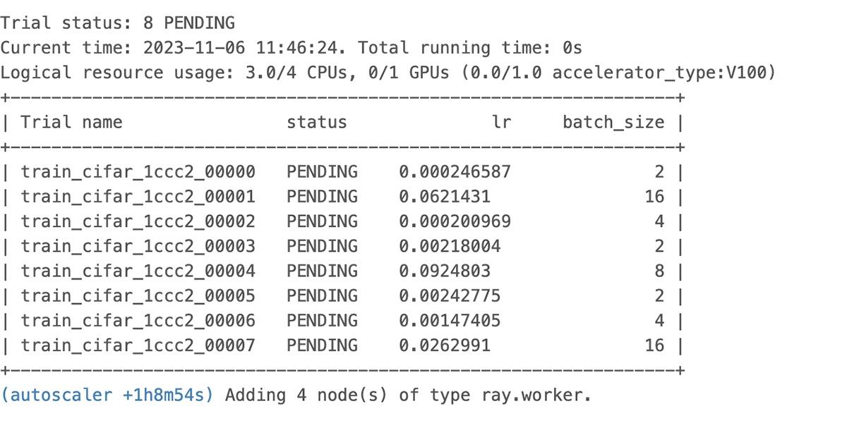
We see the autoscaler start requesting resources as shown above and the pending resource logged in the UI shown below.
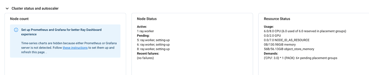
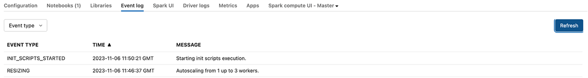
If the current demand for resources by the Ray cluster cannot be met, it initiates autoscaling of the databricks cluster as well.
Finally, we can see the run finishes the output of the Job shows that some of the bad trials were terminated early leading to compute savings
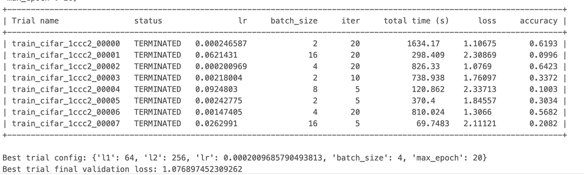
The same process works without any code change with GPU resources as well without any code change. Feel free to clone the notebook and run it in your environment:
What’s next
With the support for autoscaling Ray workload, we take one step further to tighten the integration between Ray and Databricks and help scale your dynamic workloads. Our roadmap for this integration promises even more exciting developments. Stay tuned for further updates!


