Posit AI Blog: Word Embeddings with Keras

Introduction

Word embedding is a method used to map words of a vocabulary to
dense vectors of real numbers where semantically similar words are mapped to
nearby points. Representing words in this vector space help
algorithms achieve better performance in natural language
processing tasks like syntactic parsing and sentiment analysis by grouping
similar words. For example, we expect that in the embedding space
“cats” and “dogs” are mapped to nearby points since they are
both animals, mammals, pets, etc.

In this tutorial we will implement the skip-gram model created by Mikolov et al in R using the keras package.
The skip-gram model is a flavor of word2vec, a class of
computationally-efficient predictive models for learning word
embeddings from raw text. We won’t address theoretical details about embeddings and
the skip-gram model. If you want to get more details you can read the paper
linked above. The TensorFlow Vector Representation of Words tutorial includes additional details as does the Deep Learning With R notebook about embeddings.

There are other ways to create vector representations of words. For example,
GloVe Embeddings are implemented in the text2vec package by Dmitriy Selivanov.
There’s also a tidy approach described in Julia Silge’s blog post Word Vectors with Tidy Data Principles.

Getting the Data

We will use the Amazon Fine Foods Reviews dataset.
This dataset consists of reviews of fine foods from Amazon. The data span a period of more than 10 years, including all ~500,000 reviews up to October 2012. Reviews include product and user information, ratings, and narrative text.

Data can be downloaded (~116MB) by running:

download.file("https://snap.stanford.edu/data/finefoods.txt.gz", "finefoods.txt.gz")

We will now load the plain text reviews into R.

Let’s take a look at some reviews we have in the dataset.

[1] "I have bought several of the Vitality canned dog food products ...
[2] "Product arrived labeled as Jumbo Salted Peanuts...the peanuts ... 

Preprocessing

We’ll begin with some text pre-processing using a keras text_tokenizer(). The tokenizer will be
responsible for transforming each review into a sequence of integer tokens (which will subsequently be used as
input into the skip-gram model).

library(keras)
tokenizer <- text_tokenizer(num_words = 20000)
tokenizer %>% fit_text_tokenizer(reviews)

Note that the tokenizer object is modified in place by the call to fit_text_tokenizer().
An integer token will be assigned for each of the 20,000 most common words (the other words will
be assigned to token 0).

Skip-Gram Model

In the skip-gram model we will use each word as input to a log-linear classifier
with a projection layer, then predict words within a certain range before and after
this word. It would be very computationally expensive to output a probability
distribution over all the vocabulary for each target word we input into the model. Instead,
we are going to use negative sampling, meaning we will sample some words that don’t
appear in the context and train a binary classifier to predict if the context word we
passed is truly from the context or not.

In more practical terms, for the skip-gram model we will input a 1d integer vector of
the target word tokens and a 1d integer vector of sampled context word tokens. We will
generate a prediction of 1 if the sampled word really appeared in the context and 0 if it didn’t.

We will now define a generator function to yield batches for model training.

library(reticulate)
library(purrr)
skipgrams_generator <- function(text, tokenizer, window_size, negative_samples) {
  gen <- texts_to_sequences_generator(tokenizer, sample(text))
  function() {
    skip <- generator_next(gen) %>%
      skipgrams(
        vocabulary_size = tokenizer$num_words, 
        window_size = window_size, 
        negative_samples = 1
      )
    x <- transpose(skip$couples) %>% map(. %>% unlist %>% as.matrix(ncol = 1))
    y <- skip$labels %>% as.matrix(ncol = 1)
    list(x, y)
  }
}

A generator function
is a function that returns a different value each time it is called (generator functions are often used to provide streaming or dynamic data for training models). Our generator function will receive a vector of texts,
a tokenizer and the arguments for the skip-gram (the size of the window around each
target word we examine and how many negative samples we want
to sample for each target word).

Now let’s start defining the keras model. We will use the Keras functional API.

embedding_size <- 128  # Dimension of the embedding vector.
skip_window <- 5       # How many words to consider left and right.
num_sampled <- 1       # Number of negative examples to sample for each word.

We will first write placeholders for the inputs using the layer_input function.

input_target <- layer_input(shape = 1)
input_context <- layer_input(shape = 1)

Now let’s define the embedding matrix. The embedding is a matrix with dimensions
(vocabulary, embedding_size) that acts as lookup table for the word vectors.

embedding <- layer_embedding(
  input_dim = tokenizer$num_words + 1, 
  output_dim = embedding_size, 
  input_length = 1, 
  name = "embedding"
)

target_vector <- input_target %>% 
  embedding() %>% 
  layer_flatten()

context_vector <- input_context %>%
  embedding() %>%
  layer_flatten()

The next step is to define how the target_vector will be related to the context_vector
in order to make our network output 1 when the context word really appeared in the
context and 0 otherwise. We want target_vector to be similar to the context_vector
if they appeared in the same context. A typical measure of similarity is the cosine
similarity. Give two vectors \(A\) and \(B\)
the cosine similarity is defined by the Euclidean Dot product of \(A\) and \(B\) normalized by their
magnitude. As we don’t need the similarity to be normalized inside the network, we will only calculate
the dot product and then output a dense layer with sigmoid activation.

dot_product <- layer_dot(list(target_vector, context_vector), axes = 1)
output <- layer_dense(dot_product, units = 1, activation = "sigmoid")

Now we will create the model and compile it.

model <- keras_model(list(input_target, input_context), output)
model %>% compile(loss = "binary_crossentropy", optimizer = "adam")

We can see the full definition of the model by calling summary:

_________________________________________________________________________________________
Layer (type)                 Output Shape       Param #    Connected to                  
=========================================================================================
input_1 (InputLayer)         (None, 1)          0                                        
_________________________________________________________________________________________
input_2 (InputLayer)         (None, 1)          0                                        
_________________________________________________________________________________________
embedding (Embedding)        (None, 1, 128)     2560128    input_1[0][0]                 
                                                           input_2[0][0]                 
_________________________________________________________________________________________
flatten_1 (Flatten)          (None, 128)        0          embedding[0][0]               
_________________________________________________________________________________________
flatten_2 (Flatten)          (None, 128)        0          embedding[1][0]               
_________________________________________________________________________________________
dot_1 (Dot)                  (None, 1)          0          flatten_1[0][0]               
                                                           flatten_2[0][0]               
_________________________________________________________________________________________
dense_1 (Dense)              (None, 1)          2          dot_1[0][0]                   
=========================================================================================
Total params: 2,560,130
Trainable params: 2,560,130
Non-trainable params: 0
_________________________________________________________________________________________

Model Training

We will fit the model using the fit_generator() function We need to specify the number of
training steps as well as number of epochs we want to train. We will train for
100,000 steps for 5 epochs. This is quite slow (~1000 seconds per epoch on a modern GPU). Note that you
may also get reasonable results with just one epoch of training.

model %>%
  fit_generator(
    skipgrams_generator(reviews, tokenizer, skip_window, negative_samples), 
    steps_per_epoch = 100000, epochs = 5
    )

Epoch 1/1
100000/100000 [==============================] - 1092s - loss: 0.3749      
Epoch 2/5
100000/100000 [==============================] - 1094s - loss: 0.3548     
Epoch 3/5
100000/100000 [==============================] - 1053s - loss: 0.3630     
Epoch 4/5
100000/100000 [==============================] - 1020s - loss: 0.3737     
Epoch 5/5
100000/100000 [==============================] - 1017s - loss: 0.3823 

We can now extract the embeddings matrix from the model by using the get_weights()
function. We also added row.names to our embedding matrix so we can easily find
where each word is.

Understanding the Embeddings

We can now find words that are close to each other in the embedding. We will
use the cosine similarity, since this is what we trained the model to
minimize.

library(text2vec)

find_similar_words <- function(word, embedding_matrix, n = 5) {
  similarities <- embedding_matrix[word, , drop = FALSE] %>%
    sim2(embedding_matrix, y = ., method = "cosine")
  
  similarities[,1] %>% sort(decreasing = TRUE) %>% head(n)
}

find_similar_words("2", embedding_matrix)

        2         4         3       two         6 
1.0000000 0.9830254 0.9777042 0.9765668 0.9722549 

find_similar_words("little", embedding_matrix)

   little       bit       few     small     treat 
1.0000000 0.9501037 0.9478287 0.9309829 0.9286966 

find_similar_words("delicious", embedding_matrix)

delicious     tasty wonderful   amazing     yummy 
1.0000000 0.9632145 0.9619508 0.9617954 0.9529505 

find_similar_words("cats", embedding_matrix)

     cats      dogs      kids       cat       dog 
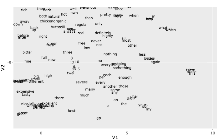
1.0000000 0.9844937 0.9743756 0.9676026 0.9624494 

The t-SNE algorithm can be used to visualize the embeddings. Because of time constraints we
will only use it with the first 500 words. To understand more about the t-SNE method see the article How to Use t-SNE Effectively.

This plot may look like a mess, but if you zoom into the small groups you end up seeing some nice patterns.
Try, for example, to find a group of web related words like http, href, etc. Another group
that may be easy to pick out is the pronouns group: she, he, her, etc.